
Text classification case study with a product-driven twist. We're building various models (logreg, RNN, transformers) and compare their quality and performance
We’re going to pretend we have an actual product we need to improve. We will explore a dataset and try out different models like logistic regression, recurrent neural networks, and transformers, looking at how accurate they are, how they are going to improve the product, how fast they work, and whether they're easy to debug and scale up.
You can read the full case study code on and see the analysis notebook with interactive charts in . GitHub Jupyter Notebook Viewer Excited? Let’s get to it! Task setting Imagine we own an E-commerce website. On this website, the seller can upload the descriptions of the items they want to sell. They also have to choose items' categories manually which may slow them down. Our task is to automate the choice of categories based on the item description. However, a wrongly automated choice is worse than no automatization, because a mistake might go unnoticed, which may lead to losses in sales. Therefore we might choose not to set an automated label if we're not sure. For this case study, we will use the , containing item descriptions and categories. Zenodo E-commerce text dataset Good or bad? How to choose the best model We will consider multiple model architectures below and it’s always a good practice to decide how to choose the best option before we start. How is this model going to impact our product? …our infrastructure? Obviously, we will have a technical quality metric to compare various models offline. In this case, we have a multi-class classification task, so let’s use a , which handles imbalanced labels well. balanced accuracy score Of course, the typical final stage of testing a candidate is AB testing - the online stage, which gives a better picture of how the customers are affected by the change. Usually, AB testing is more time-consuming than offline testing, therefore only the best candidates from the offline stage get tested. This is a case study, and we don’t have actual users, so we’re not going to cover AB testing. What else should we consider before moving a candidate forward for AB-testing? What can we think about during the offline stage to save ourselves some online testing time and make sure that we’re really testing the best possible solution? Turning technical metrics into impact-oriented metrics Balanced accuracy is great, but this score doesn’t answer the question “How exactly the model is going to impact the product?”. To find more product-oriented score we must understand how we are going to use the model. In our setting, making a mistake is worse than giving no answer, because the seller will have to notice the mistake and change the category manually. An unnoticed mistake will decrease sales and make the seller’s user experience worse, we risk losing customers. To avoid that, we’ll choose thresholds for the model’s score so that we only allow ourselves 1% of mistakes. The product-oriented metric can then be set as follows: What percentage of items can we categorise automatically if our error tolerance is only 1%? We’ll refer to this as below when selecting the best model. Find the full threshold selection code . Automatic categorisation percentage here Inference time How long does it take a model to process one request? This will roughly allow us to compare how much more resources we’ll have to maintain for a service to handle the task load if one model is selected over another. Scalability When our product is going to grow, how easy will it be to manage the growth using given architecture? By growth we might mean: more categories, higher granularity of categories longer descriptions larger datasets etc Will we have to rethink a model choice to handle the growth or a simple retrain will suffice? Interpretability How easy it will be to debug model’s errors while training and after deployment? Model size Model size matters if: we want our model to be evaluated on the client side it is so large that it could not fit into the RAM We’ll see later that both items above are not relevant, but it’s still worth considering briefly. Dataset Exploration & Cleaning What are we working with? Let’s look at the data and see if it needs cleaning up! The dataset contains 2 columns: item description and category, a total of 50.5k rows. file_name="ecommerceDataset.csv" data=pd.read_csv data.columns= print # >>>Rows, cols: Each item is assigned 1 of the 4 categories available: , , or . Here’s 1 item description example per category: Household Books Electronics Clothing & Accessories SPK Home decor Clay Handmade Wall Hanging Face Make your home more beautiful with this handmade Terracotta Indian Face Mask wall hanging, never before u can not catch this handmade thing in market. You can add this to your living room/ Entrance Lobby. Household BEGF101/FEG1-Foundation Course in English-1 BEGF101/FEG1-Foundation Course in English-1 Books Broadstar Women's Denim Dungaree Earn an all-access pass wearing dungarees by Broadstar. Made of denim, these dungarees will keep you comfy. Team them with a white or black coloured top to complete your casual look. Clothing & Accessories Caprigo Heavy Duty - 2 Feet Premium Projector Ceiling Mount Stand Bracket Electronics Missing values There’s just one empty value in the dataset, which we are going to remove. print) # # RangeIndex: 50425 entries, 0 to 50424 # Data columns : # # Column Non-Null Count Dtype # --- ------ -------------- ----- # 0 category 50425 non-null object # 1 description 50424 non-null object # dtypes: object # memory usage: 788.0+ KB data.dropna Duplicates There are however quite a lot of duplicated descriptions. Luckily all duplicates belong to one category, so we can safely drop them. repeated_messages=data .groupby .agg, n_unique_categories=)) ) repeated_messages=repeated_messages >1] print: {repeated_messages.shape}") print} out of {data.shape}") # >>>Count of repeated messages : 13979 # >>>Total number: 36601 out of 50424 After removing the duplicates we’re left with 55% of the original dataset. The dataset is well-balanced. data.drop_duplicates print print) # New dataset size: # Household 10564 # Books 6256 # Clothing & Accessories 5674 # Electronics 5308 # Name: category, dtype: int64 Description Language Note, that according to the dataset description, The dataset has been scraped from Indian e-commerce platform. The descriptions are not necessarily written in English. Some of them are written in Hindi or other languages using non-ASCII symbols or transliterated into the Latin alphabet, or use a mix of languages. Examples from category: Books यू जी सी – नेट जूनियर रिसर्च फैलोशिप एवं सहायक प्रोफेसर योग्यता … Prarambhik Bhartiy Itihas History of NORTH INDIA/வட இந்திய வரலாறு/ … To evaluate the presence of non-English words in descriptions, let’s calculate 2 scores: percentage of non-ASCII symbols in a description ASCII-score: if we consider only latin letters, what percentage of words in the description which are valid in English? Let’s say that valid English words are the ones present in trained on an English corpus. Valid English words score: Word2Vec-300 Using ASCII-score we learn that only 2.3% of the descriptions consist of more than 1% non-ASCII symbols. def get_ascii_score: total_sym_cnt=0 ascii_sym_cnt=0 for sym in description: total_sym_cnt +=1 if sym.isascii: ascii_sym_cnt +=1 return ascii_sym_cnt / total_sym_cnt data=data.apply data >>0.023 Valid English words score shows that only 1.5% of the descriptions have less than 70% of valid English words among ASCII words. w2v_eng=gensim.models.KeyedVectors.load_word2vec_format def get_valid_eng_score: description=re.sub) total_word_cnt=0 eng_word_cnt=0 for word in description.split: total_word_cnt +=1 if word.lower in w2v_eng: eng_word_cnt +=1 return eng_word_cnt / total_word_cnt data=data.apply data >>0.015 Therefore the majority of descriptions are in English or mostly in English. We can remove all other descriptions, but instead, let’s leave them as is and then see how each model handles them. Modelling Let’s split our dataset into 3 groups: Train 70% - for training the models Test 15% - for parameter and threshold choosing Eval 15% - for choosing the final model from sklearn.model_selection import train_test_split data_train, data_test=train_test_split data_test, data_eval=train_test_split data_train.shape, data_test.shape, data_eval.shape # >>>, , ) Baseline model: bag of words + logistic regression It’s helpful to do something straightforward and trivial at first to get a good baseline. As a baseline let’s create a bag of words structure based on the train dataset. Let’s also limit the dictionary size to 100 words. count_vectorizer=CountVectorizer x_train_baseline=count_vectorizer.fit_transform y_train_baseline=data_train x_test_baseline=count_vectorizer.transform y_test_baseline=data_test x_train_baseline=x_train_baseline.toarray x_test_baseline=x_test_baseline.toarray I’m planning to use logistic regression as a model, so I need to normalize counter features before training. ss=StandardScaler x_train_baseline=ss.fit_transform x_test_baseline=ss.transform lr=LogisticRegression lr.fit balanced_accuracy_score) # >>>0.752 Multi-class logistic regression showed 75.2% balanced accuracy. This is a great baseline! Although the overall classification quality is not great, the model can still give us some insights. Let’s look at the confusion matrix, normalized by the number of predicted labels. The X-axis denotes the predicted category, and the Y-axis - the real category. Looking at each column we can see the distribution of real categories when a certain category was predicted. For example, is frequently confused with . But even this simple model can capture quite precisely. Electronics Household Clothing & Accessories Here are feature importances when predicting category: Clothing & Accessories Top-6 most contributing words towards and against category: Clothing & Accessories women 1.49 book -2.03 men 0.93 table -1.47 cotton 0.92 author -1.11 wear 0.69 books -1.10 fit 0.40 led -0.90 stainless 0.36 cable -0.85 RNNs Now let’s consider more advanced models, designed specifically to work with sequences - . and are common advanced layers to fight the exploding gradients that occur in simple RNNs. recurrent neural networks GRU LSTM We’ll use library to tokenize descriptions, and build and train a model. pytorch First, we need to transform texts into numbers: Split descriptions into words Assign an index to each word in the corpus based on the training dataset Reserve special indices for unknown words and padding Transform each description in train and test datasets into vectors of indices. The vocabulary we get from simply tokenizing the train dataset is large - almost 90k words. The more words we have, the larger the embedding space the model has to learn. To simplify the training, let’s remove the rarest words from it and leave only those that appear in at least 3% of descriptions. This will truncate the vocabulary down to 340 words. CorpusDictionary here corpus_dict=util.CorpusDictionary corpus_dict.truncate_dictionary data_train=corpus_dict.transform data_test=corpus_dict.transform print) # 28453 .apply)) # >>>9388 print, q=0.95))) # >>>352 Next - we need to transform target categories into 0-1 vectors to compute loss and perform back-propagation on each training step. def get_target: target= * total_labels target=1 return target data_train=data_train.apply data_test=data_test.apply Now we’re ready to create a custom Dataset and Dataloader to feed into the model. Find full implementation . pytorch PaddedTextVectorDataset here ds_train=util.PaddedTextVectorDataset ds_test=util.PaddedTextVectorDataset train_dl=DataLoader test_dl=DataLoader Finally, let’s build a model. The minimal architecture is: embedding layer RNN layer linear layer activation layer Starting with small values of parameters and no regularisation, we can gradually make the model more complicated until it shows strong signs of over-fitting, and then balance regularisation . class GRU: def __init__: super.__init__ self.vocab_size=vocab_size self.embedding_dim=embedding_dim self.n_hidden=n_hidden self.n_out=n_out self.emb=nn.Embedding self.gru=nn.GRU self.dropout=nn.Dropout self.out=nn.Linear def forward: batch_size=sequence.size self.hidden=self._init_hidden embs=self.emb embs=pack_padded_sequence gru_out, self.hidden=self.gru gru_out, lengths=pad_packed_sequence dropout=self.dropout output=self.out return F.log_softmax def _init_hidden: return Variable)) We’ll use optimizer and as a loss function. Adam cross_entropy vocab_size=len emb_dim=4 n_hidden=15 n_out=len model=GRU opt=optim.Adam, 1e-2) util.fit # >>>Train loss: 0.3783 # >>>Val loss: 0.4730 This model showed 84.3% balanced accuracy on eval dataset. Wow, what a progress! Introducing pre-trained embeddings The major downside to training the RNN model from scratch is that it has to learn the meaning of the words itself - that is the job of the embedding layer. Pre-trained models are available to use as a ready-made embedding layer, which reduces the number of parameters and adds a lot more meaning to tokens. Let’s use one of the models available in - . word2vec word2vec pytorch glove, dim=300 We only need to make minor changes to the Dataset creation - we now want to create a vector of pre-defined indexes for each description, and the model architecture. glove ds_emb_train=util.PaddedTextVectorDataset ds_emb_test=util.PaddedTextVectorDataset dl_emb_train=DataLoader dl_emb_test=DataLoader import torchtext.vocab as vocab glove=vocab.GloVe class LSTMPretrained: def __init__: super.__init__ self.emb=nn.Embedding.from_pretrained self.emb.requires_grad_=False self.embedding_dim=300 self.n_hidden=n_hidden self.n_out=n_out self.lstm=nn.LSTM self.dropout=nn.Dropout self.out=nn.Linear def forward: batch_size=sequence.size self.hidden=self.init_hidden embs=self.emb embs=pack_padded_sequence lstm_out, =self.lstm lstm_out, lengths=pad_packed_sequence dropout=self.dropout output=self.out return F.log_softmax def init_hidden: return Variable)) And we’re ready to train! n_hidden=50 n_out=len emb_model=LSTMPretrained opt=optim.Adam, 1e-2) util.fit Now we’re getting 93.7% balanced accuracy on eval dataset. Woo! BERT Modern state-of-the-art models for working with sequences are transformers. However, to train a transformer from scratch, we would need massive amounts of data and computational resources. What we can try here - is to fine-tune one of the pre-trained models to serve our purpose. To do this we need to download a and add dropout and linear layer to get the final prediction. It’s recommended to train a tuned model for 4 epochs. I trained only 2 extra epochs to save time - it took me 40 minutes to do that. pre-trained BERT model from transformers import BertModel class BERTModel: def __init__: super.__init__ self.l1=BertModel.from_pretrained self.l2=nn.Dropout self.l3=nn.Linear def forward: output_1=self.l1 output_2=self.l2 output=self.l3 return output ds_train_bert=bert.get_dataset, list, max_vector_len=64 ) ds_test_bert=bert.get_dataset, list, max_vector_len=64 ) dl_train_bert=DataLoader, batch_size=batch_size) dl_test_bert=DataLoader, batch_size=batch_size) b_model=bert.BERTModel b_model.to) def loss_fn: return torch.nn.BCEWithLogitsLoss optimizer=optim.AdamW, lr=2e-5, eps=1e-8) epochs=2 scheduler=get_linear_schedule_with_warmup bert.fit torch.save Training log: 2024-02-29 19:38:13.383953 Epoch 1 / 2 Training... 2024-02-29 19:40:39.303002 step 40 / 305 done 2024-02-29 19:43:04.482043 step 80 / 305 done 2024-02-29 19:45:27.767488 step 120 / 305 done 2024-02-29 19:47:53.156420 step 160 / 305 done 2024-02-29 19:50:20.117272 step 200 / 305 done 2024-02-29 19:52:47.988203 step 240 / 305 done 2024-02-29 19:55:16.812437 step 280 / 305 done 2024-02-29 19:56:46.990367 Average training loss: 0.18 2024-02-29 19:56:46.990932 Validating... 2024-02-29 19:57:51.182859 Average validation loss: 0.10 2024-02-29 19:57:51.182948 Epoch 2 / 2 Training... 2024-02-29 20:00:25.110818 step 40 / 305 done 2024-02-29 20:02:56.240693 step 80 / 305 done 2024-02-29 20:05:25.647311 step 120 / 305 done 2024-02-29 20:07:53.668489 step 160 / 305 done 2024-02-29 20:10:33.936778 step 200 / 305 done 2024-02-29 20:13:03.217450 step 240 / 305 done 2024-02-29 20:15:28.384958 step 280 / 305 done 2024-02-29 20:16:57.004078 Average training loss: 0.08 2024-02-29 20:16:57.004657 Validating... 2024-02-29 20:18:01.546235 Average validation loss: 0.09 Finally, fine tuned BERT model shows whopping 95.1% balanced accuracy on eval dataset. Choosing our winner We’ve already established a list of considerations to look at to make a final well-informed choice. Here are charts showing measurable parameters: Although fine-tuned BERT is leading in quality, RNN with pre-trained embedding layer is a close second, only falling behind by 3% of automatic category assignments. LSTM+EMB On the other hand, the inference time of fine-tuned BERT is 14 times longer than . This will add up in backend maintenance costs which will probably outweigh the benefits fine-tuned brings over . LSTM+EMB BERT LSTM+EMB As for interoperability, our baseline logistic regression model is by far the most interpretable and any neural network loses to it in this regard. At the same time, the baseline is probably the least scalable - adding categories will decrease the already low quality of the baseline. Even though BERT seems like the superstar with its high accuracy, we end up going with the RNN with a pre-trained embedding layer. Why? It's pretty accurate, not too slow, and doesn't get too complicated to handle when things get big. Hope you enjoyed this case study. Which model would you have chosen and why?
United States Latest News, United States Headlines
Similar News:You can also read news stories similar to this one that we have collected from other news sources.
 How Amazon Web Services' AI, machine learning technology is shaping NFL's futureAmazon Web Services' Head of Sports Julie Souza couldn't be happier with how the 2023 NFL season went. The NFL used its AI and machine learning technology to make the game better.
Read more »
 Unmasking the Universe With AI: How Machine Learning Unravels Black Hole MysteriesScience, Space and Technology News 2024
Read more »
 Researchers leverage machine learning to find surprising temperature-genome correlationA recent study by researchers uncover clues in extremophiles' genomes, revealing genomic shifts and hinting at astrobiological implications.
Read more »
 3 Myths About Machine Learning in Health CareMachine learning will dramatically improve health care. There are already myriad impactful ML health care applications from imaging to predicting readmissions to the back office. But there are also high-profile, expensive efforts that have not achieved their goals.
Read more »
 The role of machine learning and computer vision in ImageomicsA new field promises to usher in a new era of using machine learning and computer vision to tackle small and large-scale questions about the biology of organisms around the globe.
Read more »
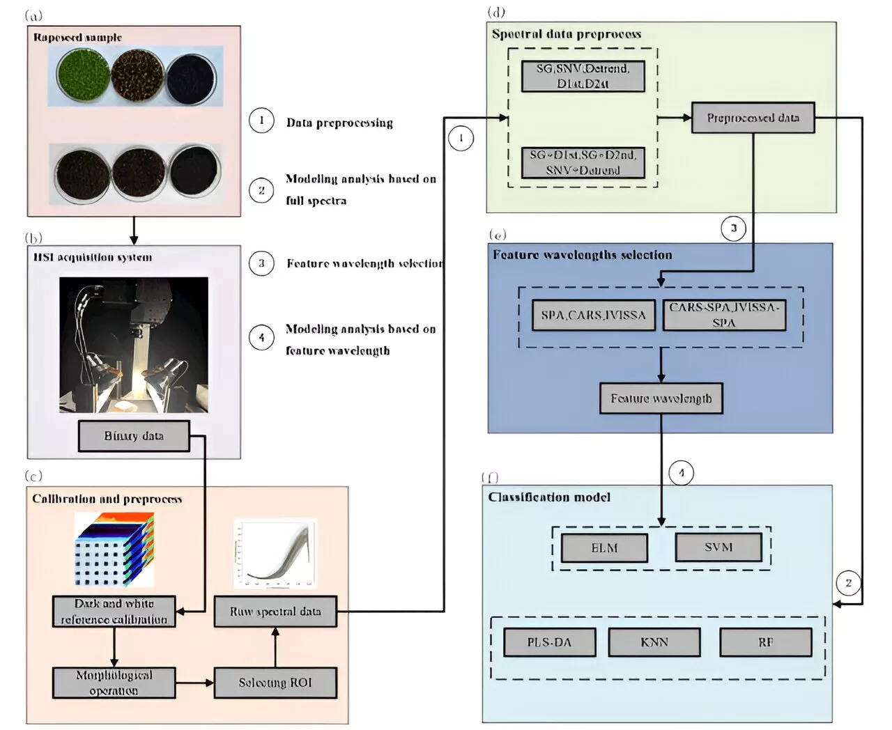 Enhancing rapeseed maturity classification with hyperspectral imaging and machine learningRapeseed oil, a vital oilseed crop facing growing global demand, encounters a significant challenge in achieving uniform seed maturity, owing to asynchronous flowering. Traditional maturity assessment methods are limited by their destructive nature.
Read more »